[Guide] Nowadays, machine learning is shifting from manual design models to automatic optimization workflows. Tools such as H20, TPOT, and auto-sklearn have been widely used. These libraries and random search methods are dedicated to finding the most suitable model for the data set, so as to simplify the model selection and tuning process without any manual intervention. However, feature engineering, as the most valuable part of the machine learning process, is almost always done manually.
In this article, we introduce the basic knowledge by citing a data set as an example, and introduce an example of feature engineering automation based on Featuretools Python library.
Preface
Feature engineering can also be called feature construction, which is the process of training machine learning models by constructing new features based on existing data. It can be said that this link is more important than the specific model we use, because the machine learning algorithm will only learn based on the data we provide it, so it is extremely important to construct features related to the target task (see the paper "A Few Useful Things to Know about Machine Learningâ€).
Paper link:
https://homes.cs.washington.edu/~pedrod/papers/cacm12.pdf
Generally speaking, feature engineering is a long manual process that relies on domain knowledge, intuition and data manipulation. This process is extremely monotonous, and the final characteristic result will be limited by human subjectivity and time. Automatic feature engineering aims to help data scientists automatically construct candidate features based on data sets and select the most suitable features for training.
Basic knowledge of feature engineering
Feature engineering means constructing additional features based on existing data. The data to be analyzed is often distributed in multiple associated tables. Feature engineering needs to extract information from data, and then integrate it into a single table for training machine learning models.
Feature construction is a very time-consuming process, because each new feature needs to go through several steps to construct, especially those that require multiple tables of information. We can combine the operations of these feature constructions into two categories: "transformation" and "aggregation". Let's use a few examples to understand these concepts.
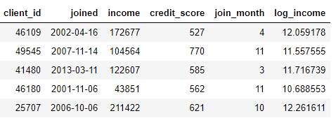
"Conversion" applies to a single table. This link constructs new features based on one or more existing data columns. For example, now we have the following customer data table:

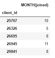
We can construct new features by looking up the month in the joined column or taking the natural logarithm of the income column. These are all "conversion" operations, because they only use information from a table.
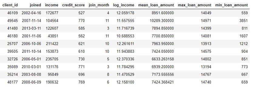
On the other hand, "aggregation" requires cross-table operations, and group observations based on a one-to-many relationship, and then perform data statistics. For example, if we have another table about customer loan information, in which each customer may have multiple loans, then we can calculate the average, maximum, and minimum statistics of each customer's loan amount.
This process includes grouping loan data tables according to different users, calculating aggregated statistics, and then integrating the results into customer data. Here is the code we use Pandas to perform this process in Python:
importpandasaspd#Grouploansbyclientidandcalculatemean,max,minofloansstats=loans.groupby('client_id')['loan_amount'].agg(['mean','max','min'])stats.columns=['mean_loan_amount','max_loan_amount' ,'min_loan_amount']#Mergewiththeclientsdataframestats=clients.merge(stats,left_on='client_id',right_index=True,how='left')stats.head(10)
These operations themselves are not difficult, but if we have hundreds of variables distributed in dozens of tables, it will be more difficult to complete this process manually. Ideally, we want to find a solution that can automatically perform the conversion and aggregation of multiple tables, and integrate the resulting data into one table. Although Pandas is a great resource, the amount of data manipulation that we need to complete manually is still huge!
â–ŒFeaturetools
Fortunately, the feature tool is exactly the solution we are looking for. This open source Python library can automatically create features based on a set of related tables. The feature tool is based on "Deep Feature Synthesis (DFS)". This method sounds much more advanced than it itself (the reason why it is called "Deep Feature Synthesis" is not because of the use of deep learning, but because it is superimposed Multiple features).
Deep feature synthesis superimposes multiple conversion and aggregation operations, which are called feature primitives in the feature tool lexicon, and are used to construct features from multiple tables of data. Like most methods in machine learning, this is a complex method based on simple concepts. By learning one building block at a time, we can understand this powerful method well.
First, let's take a look at the data in the example. We have seen some of the data sets mentioned above, and all the tables are as follows:
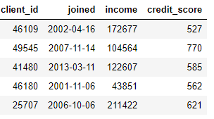
clients: Basic information about the clients of a credit union. Each customer only corresponds to one row of data in the table.
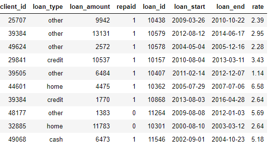
loans: Loans under the customer's name. Each loan only corresponds to one row of data in the table, but there may be multiple loans under each customer's name.
payments: the amount of loan repayment. Each payment corresponds to only one row of data, but each loan may be paid in multiples.
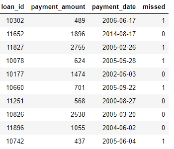
If we have a machine learning task, such as predicting whether a certain customer will pay off a future loan, we need to integrate all the information about the customer into one table. These tables are related to each other through the variables client_id and loan_id, and we can use a series of transformations and aggregations to manually complete this process. However, we will soon discover that we can use feature tools to automate this process.
â–ŒEntity and entity set
First, we must introduce the two concepts of feature tools: entity and entity set. Simply put, an entity is a table (that is, a DataFrame in Pandas). An entity set refers to a collection of multiple tables and the relationship between them. We can think of the entity set as a Python data structure with its own methods and attributes.
We can create an empty entity set in the feature tool as follows:
importfeaturetoolsasft#Createnewentitysetes=ft.EntitySet(id='clients')
Now we are going to merge multiple entities. Each entity must have an index, that is, a data column with all elements unique. In other words, each value in the index column can only appear once in the table.
The index of the clients data frame (dataframe) is client_id, because each client only corresponds to one row of data in the table. We can add an indexed entity to an entity set through the following syntax:
#Createanentityfromtheclientdataframe#Thisdataframealreadyhasanindexandatimeindexes=es.entity_from_dataframe(entity_id='clients',dataframe=clients,index='client_id',time_index='joined')
The loans data frame also has a unique index loan_id, and the syntax for adding it to the entity set is the same as the syntax for processing clients. However, there is no unique index in the payments data frame. If we want to add this entity to the entity set, we need to make make_index = True and specify an index name. Although the feature tool can automatically infer the data type of each column in the entity, we can also overwrite it by passing the data type dictionary into the parameter variable_types.
#Createanentityfromthepaymentsdataframe#Thisdoesnotyethaveauniqueindexes=es.entity_from_dataframe(entity_id='payments',dataframe=payments,variable_types={'missed':ft.variable_types.Categorical},make_index=True,index='payment_id',time_index='payment
For this data frame, although missed is an integer, it is not a numeric variable, because it can only take two discrete values, so we let the feature tool treat it as a categorical variable. After adding all the data frames to the entity set, we see:
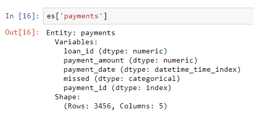
According to the correction scheme we specified, the types of these columns have been correctly identified. In the next step, we need to specify the association between the tables in the entity set.
â–ŒThe association between tables
The best way to study the relationship between two tables is to make an analogy with the parent-child relationship. This is a one-to-many relationship: each father may have multiple children. From the perspective of the table, each row in the parent table corresponds to a father, but the child table may have multiple rows of data, just like multiple children of the same father.
For example, in our data set, clients is the parent table of loans. Each customer corresponds to only one row of data in the clients table, but may correspond to multiple rows of data in the loans table. Similarly, loans is the parent table of payments, because each loan may contain multiple payments. The parent table is connected to the child table through shared variables. When performing aggregation operations, we classify the child tables according to the variables of the parent table and calculate the statistics of each child table.
To indicate the association in the feature tool, we only need to specify the variable that connects the two tables. Table clients and table loans are related through variable client_id, table loans and table payments are related through loan_id. You can create an association and add it to the entity set through the following syntax:
#Relationshipbetweenclientsandpreviousloansr_client_previous=ft.Relationship(es['clients']['client_id'],es['loans']['client_id'])#Addtherelationshiptotheentitysetes=es.add_relationship(r_client_previous)#Relationrbetweenpaymentes=Relationrbetweenprevious loans']['loan_id'],es['payments']['loan_id'])#Addtherelationshiptotheentitysetes=es.add_relationship(r_payments)es
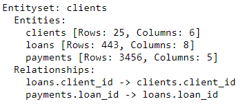
The entity set now includes three entities and the relationships that connect these entities. After adding entities and marking the association, our entity set is complete and ready to construct new features.
â–ŒFeature primitives
Before formal deep feature synthesis, we need to understand the concept of feature primitives. We already know what feature primitives are, but we only know what names are used to call them. The following is the basic operation when we construct a new feature:
Aggregation: A series of operations based on the association (one-to-many) between the parent table and the child table, that is, the child table is grouped according to the parent table and its statistics are calculated. For example, group the loan table according to client_id and find the largest loan amount for each client.
Conversion: An operation performed on one or more columns in a table. For example, calculating the difference between two columns in a table or calculating the absolute value of a column.
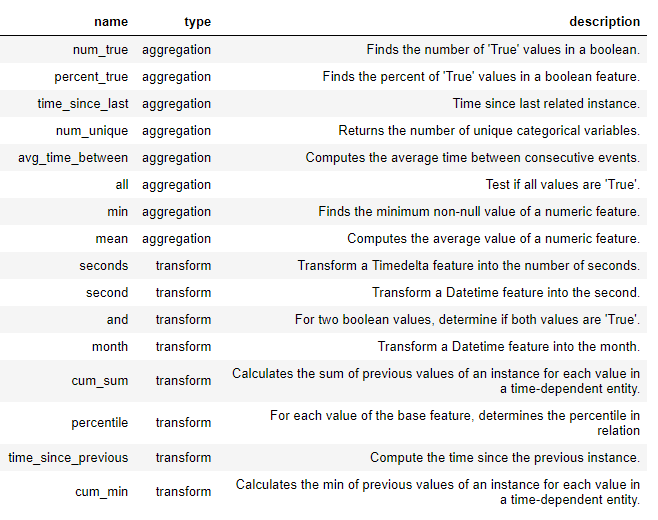
In the feature tool, we can construct new features by using a single primitive or superimposing multiple primitives. The following is a list of some feature primitives in the feature tool (we can also customize the primitives):
â–ŒFeature primitives
These primitives can be used alone or combined to construct new features. According to specific primitives, we can use the ft.dfs function (ie, depth feature synthesis) to construct features. We pass the selected trans_primitives (transition) and agg_primitives (aggregation) into entityset (entity set) and target_entity (target entity), that is, the table to which we want to add features:
#Createnewfeaturesusingspecifiedprimitivesfeatures,feature_names=ft.dfs(entityset=es,target_entity='clients',agg_primitives=['mean','max','percent_true','last'],trans_primitives=['years','month', 'subtract','divide'])
The result is a customer data frame with new features (because we treat users as target_entity). For example, if we know the month each user joined, this can be used as a conversion feature primitive:
We also have many aggregation primitives, such as the average payment per customer:

Although we only listed a part of the feature primitives, in fact, the feature tool constructs many new features by combining and superimposing these primitives.

The complete data frame contains 793 new features!
â–ŒDeep feature synthesis
Now we are all ready to understand deep feature synthesis. In fact, we have used deep feature synthesis before executing the function! Deep feature refers to the feature obtained by superimposing multiple primitives, and deep feature synthesis refers to the process of constructing these features. The depth of a depth feature is the number of primitives used to construct the feature.
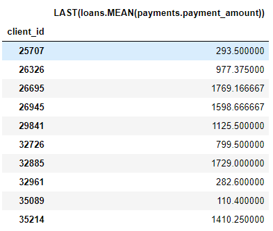
For example, the MEAN (payments.payment_amount) column is a depth feature with a depth of 1, because it uses only one aggregation primitive in the construction process. LAST(loans(MEAN(payments.payment_amount)) is a feature with a depth of 2. It is composed of two aggregate primitives superimposed: LAST is superimposed on MEAN. This feature represents the average value of the customer's most recent payment.
We can stack features to any depth we want, but in fact, I have never used features with a depth greater than 2. It is difficult to explain this point clearly, but I encourage interested people to try further exploration.
We don't need to manually specify feature primitives, feature tools can help us automatically select features. To this end, we also use the ft.dfs function to call without passing in any feature primitives:
#Performdeepfeaturesynthesiswithoutspecifyingprimitivesfeatures,feature_names=ft.dfs(entityset=es,target_entity='clients',max_depth=2)features.head()

The feature tool constructs many new features for us to use. Although this process can automatically construct new features, it will not replace the data scientist because we need to know how to use these features. For example, if our goal is to predict whether a certain customer will repay the loan, then we need to find the feature that is most relevant to the specified result. In addition, if we have domain knowledge, we can use domain knowledge to select specific feature primitives, or obtain seed features from candidate features through deep feature synthesis.
â–ŒNext
Automatic feature engineering solves one problem, but it also creates another problem: too many features. Although it is difficult to say which features are important before fitting the model, certainly not all features are related to the target task. Moreover, too many features may lead to poor model performance, because less important features will affect those more important features.
The problems caused by too many features are again recognized as the "curse of dimensionality." For the model, the number of features has increased (that is, the dimensionality of the data has increased), and it will become more difficult to learn the mapping rules between features and targets. In fact, the amount of data required to make the model perform well has an exponential relationship with the number of features.
The "curse of dimensionality" can be mitigated by feature dimensionality reduction (also known as feature selection): this is a process of eliminating irrelevant features. We can do this in a variety of ways: principal component analysis (PCA), SelectKBest, using the feature importance of the model, or using deep neural networks to automate coding. Compared with the content to be discussed today, it is more appropriate to start a separate article for feature dimensionality reduction. So far, we already know how to use feature tools to easily construct a large number of features from many data tables!
to sum up
Like many topics in machine learning, automatic feature engineering based on feature tools is a complex method based on simple concepts. Based on the concepts of entity set, entity and association, feature tools can construct new features through deep feature synthesis. In-depth feature synthesis superimposes the "aggregate" feature primitives that include one-to-many associations between tables. The "conversion" function is used for one or more columns of data in a single table to construct new features from multiple tables.
In subsequent articles, the AI ​​Technology Base Camp will also introduce how to use this technology in practical applications (such as Kaggle competitions). The quality of the model depends on the data we provide for it, and automatic feature engineering helps to make the feature construction process more efficient. I hope that the automatic feature engineering introduced in this article can help you.
For more information about feature tools, including more advanced application methods, you can view the online documentation.
Full-Range Speaker,Sensitivity Speaker,Fullrange Speaker,3 Inch Full-Range Speaker
Guangzhou BMY Electronic Limited company , https://www.bmy-speakers.com
