
Concentration is the essence. It is easy to write thick, but it is very difficult to write thin. There are so many classic machine learning algorithms. If they can grasp their core essence, they will be very helpful for understanding and memory, and it will also make you more likely to pass the interview. In this article, SIGAI will summarize each typical machine learning algorithm in one sentence to help you grasp the essence of the problem and strengthen understanding and memory. Let’s get started.
Bayesian classifier

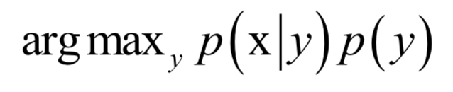
Core: Determine the sample as the class with the largest posterior probability

The Bayesian classifier directly uses the Bayesian formula to solve the classification problem. Assuming that the feature vector of the sample is x and the category label is y, according to the Bayesian formula, the conditional probability (posterior probability) that the sample belongs to each class is:

The denominator p(x) is the same for all classes. The classification rule is to classify the sample into the class with the largest posterior probability. There is no need to calculate the accurate probability value. You only need to know which class has the largest probability. The denominator can be ignored. The discriminant function of the classifier is:
When implementing a Bayesian classifier, it is necessary to know the conditional probability distribution p(x|y) of each class, which is the prior probability. It is generally assumed that the sample obeys a normal distribution. During training, the parameters of the prior probability distribution are determined, and the maximum likelihood estimation is generally used, that is, to maximize the log-likelihood function.
Bayesian sub-classifier is a generative model that can handle multiple classification problems and is a nonlinear model.
Decision tree

Core: a set of nested decision rules

The decision tree is essentially a set of nested if-else decision rules, which is a piecewise constant function mathematically, which corresponds to the division of space by a plane parallel to the coordinate axis. Decision rules are commonly used methods when humans deal with many problems. These rules are summed up through experience, and these rules of decision trees are automatically learned through training samples. The following is a simple decision tree and the result of its division of space:
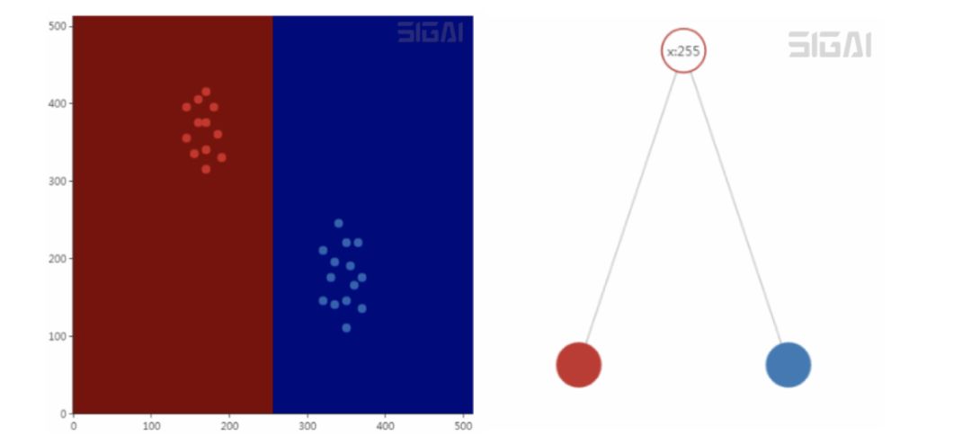
When training, find the best split by maximizing Gini or other indicators. The decision tree can input the importance of each component of the feature vector.
Decision tree is a discriminant model that supports both classification problems and regression problems. It is a non-linear model (piecewise linear functions are not linear). It naturally supports multiple classification problems.
kNN algorithm

Core: template matching, classify the sample into the class of the sample that is most similar to it

The kNN algorithm essentially uses the idea of ​​template matching. To determine the category of a sample, you can calculate the distance between it and all training samples, and then find the k samples that are closest to the sample, count the categories of these samples for voting, and the category with the most votes is the classification result. The following figure is a schematic diagram of the kNN algorithm:
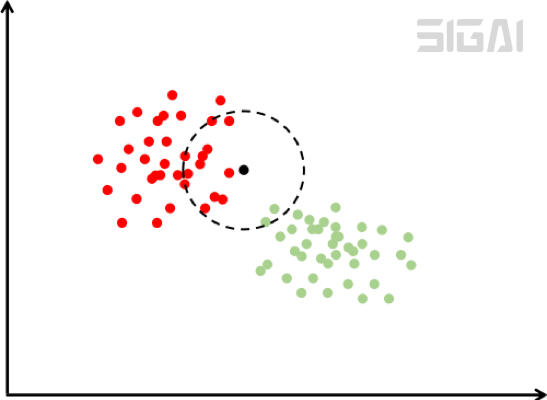
In the picture above, there are two types of samples, red and green. For the sample to be classified, that is, the black point in the figure, search for a part of the training sample closest to the sample. In the figure, it is all samples within a certain circle centered on this rectangular sample. Then count the categories to which these samples belong. Here there are 12 red dots and 2 circles, so this sample is judged as red.
The kNN algorithm is a discriminative model that supports classification problems and regression problems, and is a non-linear model. It naturally supports multiple classification problems. The kNN algorithm has no training process and is an example-based algorithm.
PCA

Core: linear projection to the direction of the smallest reconstruction error (the largest variance)

PCA is a method of data dimensionality reduction and correlation removal. It uses linear transformation to project a vector into a low-dimensional space. To project a vector is to multiply the vector by a matrix to get the result vector. This is the linear transformation described in linear algebra:
y = Wx
The dimensionality reduction must ensure that the projection in the low-dimensional space can approximate the original vector well, that is, the reconstruction error is minimized. The figure below is a schematic diagram of principal component projection:
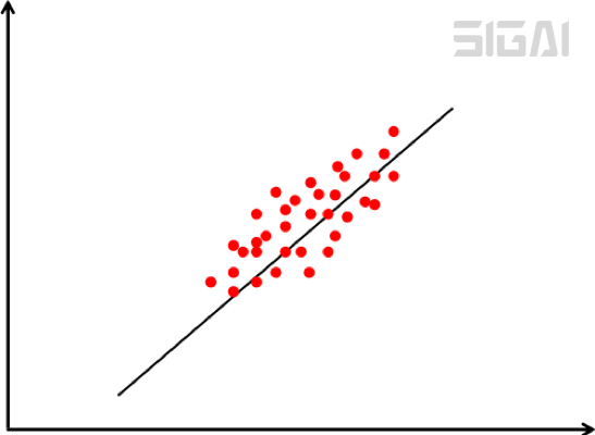
In the above figure, the samples are represented by red dots, and the inclined straight line is their main direction of change. Projecting the data onto this straight line completes the dimensionality reduction of the data, reducing the data from 2 dimensions to 1 dimension. The optimization problem solved when calculating the best projection direction is:
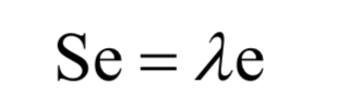
Finally, it boils down to finding the eigenvalues ​​and eigenvectors of the covariance matrix:
PCA is an unsupervised learning algorithm. It is a linear model and cannot be directly used for classification and regression problems.
LDA

Core: Linear projection to the direction of maximizing the difference between classes and minimizing the difference within classes

The basic idea of ​​linear discriminant analysis is to minimize the difference between samples of the same type and maximize the difference between samples of different types through linear projection. The specific method is to find a projection matrix W to a low-dimensional space, and the new vector obtained after the eigenvector x of the sample is projected:
y = Wx
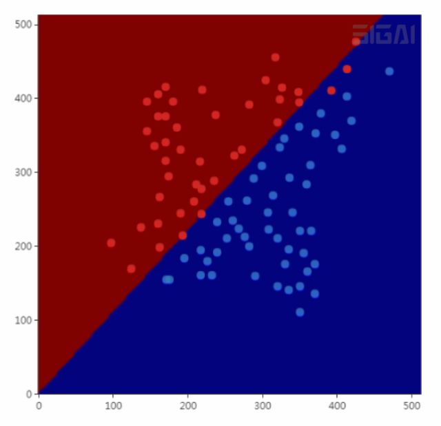
The result vector difference after the same type of projection is as small as possible, and the difference of samples of different types is as large as possible. Intuitively, after this projection, samples of the same type come in and gather together, and samples of different types are as far away as possible. The following figure is a schematic diagram of this projection:
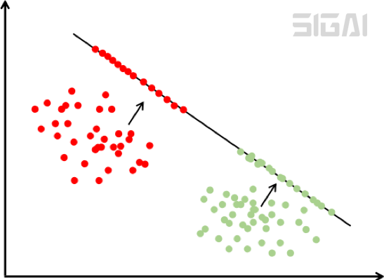
The feature vector in the above figure is two-dimensional. We project to a one-dimensional space, that is, a straight line. After projection, these points are located on the straight line. In the above figure, there are two types of samples, and the two types of samples are effectively separated by a straight line projection to the upper right. The green sample is located in the lower half of the line after projection, and the red sample is located in the upper half of the line after projection.
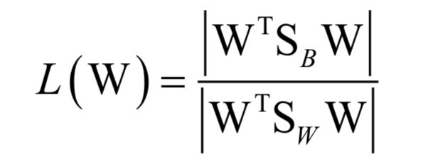
The optimization goal during training is the ratio of the difference between the classes to the difference within the classes:
Finally, it comes down to solving the eigenvalues ​​and eigenvectors of the matrix:
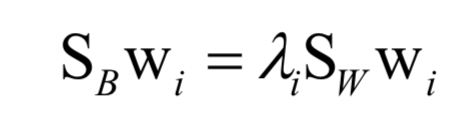
LDA is a supervised machine learning algorithm that uses sample label values ​​in the calculation process. This is a discriminative model and also a linear model. LDA cannot be directly used for classification and regression problems. To classify the reduced-dimensional vectors, other algorithms, such as kNN, are needed.
LLE (Manifold Learning)

Core: Approximately reconstruct the sample with a linear combination of neighbors of a sample point, and maintain this linear combination relationship after projecting the sample into a low-dimensional space

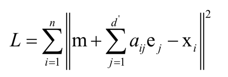
Local linear embedding (LLE for short) projects high-dimensional data into low-dimensional space and maintains the local linear relationship between data points. The core idea is that each point can be approximated by a linear combination of multiple points close to it. After projecting into a low-dimensional space, this linear reconstruction relationship must be maintained and the same reconstruction coefficients must be maintained.
The first step of the algorithm is to solve the reconstruction coefficients. Each sample point xi can be linearly represented by its neighbors, that is, the following optimization problem:
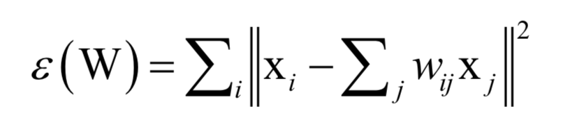
In this way, the linear combination coefficient between each sample point and its neighbor nodes can be obtained. Next, take this combination coefficient as a known quantity, and solve the following optimization problem to complete the vector projection:
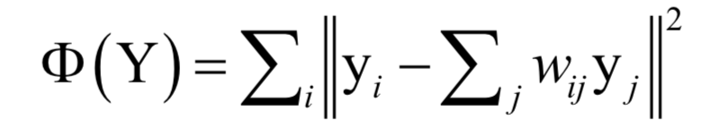
In this way, the vector y can be obtained, which is the vector after projection.
LLE is an unsupervised machine learning algorithm. It is a non-linear dimensionality reduction algorithm and cannot be directly used for classification or regression problems.
Isometric mapping (manifold learning)

Core: The relative distance relationship is maintained after the sample is projected into the low-dimensional space

Isometric mapping uses the idea of ​​geodesic in differential geometry. It hopes that the data can maintain the geodesic distance on the manifold after mapping to low-dimensional space. The so-called geodesic is the arc corresponding to the shortest distance between two points on the surface of the earth. Intuitively, after projecting into a low-dimensional space, the relative distance relationship must be maintained, that is, points that are far away before projection are farther away after projection, and points that are close before projection are closer after projection.
We can use the projection of the three-dimensional spherical map of the globe into a two-dimensional flat map to understand:

After being projected into a flat map:

On the globe before the projection, the United States is far away from China, and Thailand is nearer to China. After the projection is made into a flat map, the relative distance must be maintained.
Isometric mapping is an unsupervised learning algorithm and a non-linear dimensionality reduction algorithm.
Artificial neural networks

Core: a multi-layered composite function

The artificial neural network is essentially a multi-layer composite function:
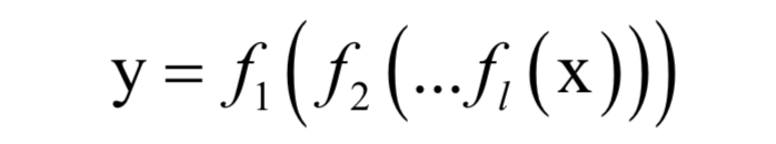
It implements the mapping from vector x to vector y. Since a non-linear activation function f is used, this function is a non-linear function.
The problem solved during neural network training is not a convex optimization problem. The back-propagation algorithm is derived from the chain rule of derivation of multiple compound functions.
The standard neural network is a supervised learning algorithm and a non-linear model. It can be used for both classification problems and regression problems. It naturally supports multi-classification problems.
Support Vector Machines

Core: Linear classifier that maximizes the classification interval (without considering the kernel function)

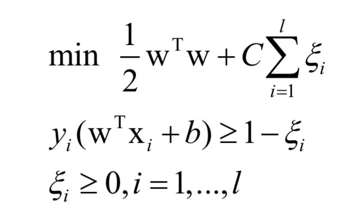
The goal of the support vector machine is to find a classification hyperplane, which can not only correctly classify each sample, but also make the distance between the closest sample to the hyperplane in each class of samples and the hyperplane as far as possible.

The original problem solved during training is:
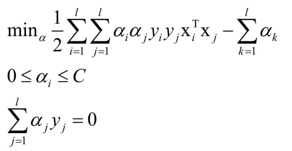
The dual problem is:
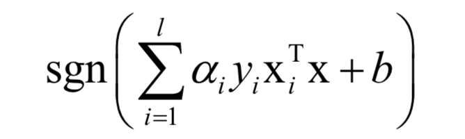
For classification problems, the prediction function is:
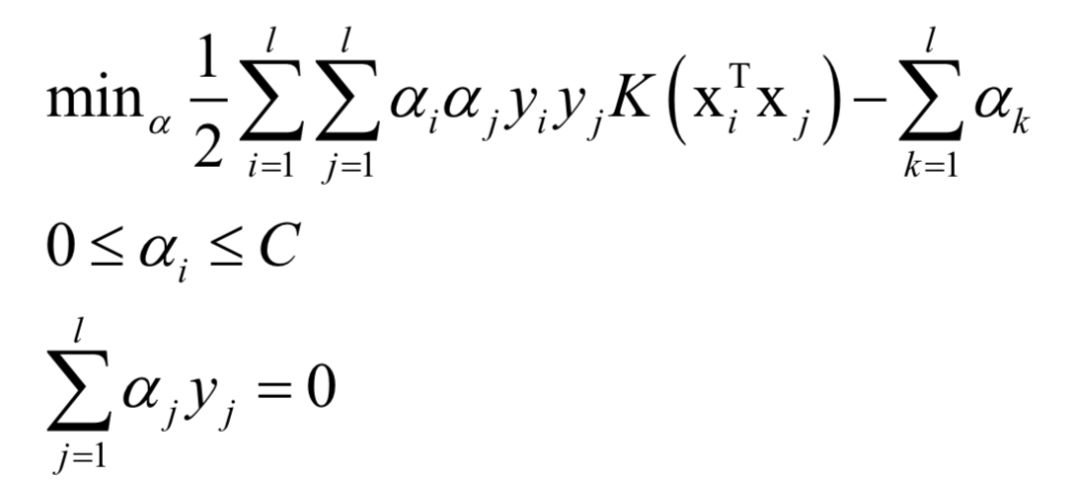
If a nonlinear kernel function is not used, SVM is a linear model. After using the kernel function, the dual problem solved during SVM training is:
For classification problems, the prediction function is:
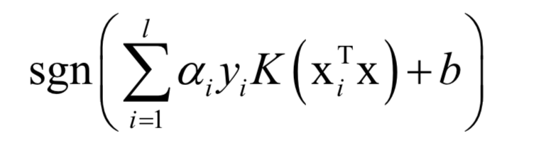
If a nonlinear kernel is used, SVM is a nonlinear model.
The problem to be solved during training is a convex optimization problem. The solution uses the SMO algorithm, which is a divide-and-conquer method in which two variables are selected for optimization each time, and the other variables remain unchanged. The basis for selecting optimized variables is the KKT condition. The optimization of these two variables is a quadratic function extreme value problem, and the formula solution can be directly obtained.
SVM is a discriminative model. It can be used for both classification problems and regression problems. The standard SVM can only support two classification problems, and a combination of multiple classifiers can solve multi-classification problems.
logistic regression

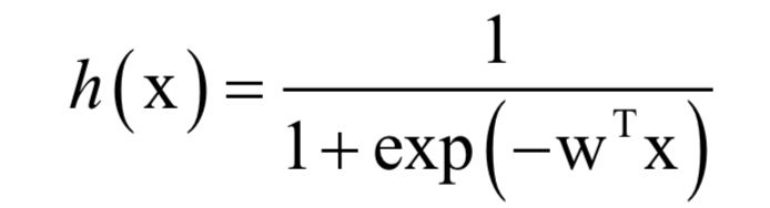
Core: directly estimate the probability that it belongs to a positive and negative sample from the sample

By first weighting the vector linearly, and then calculating the logistic function, the probability value between [0,1] can be obtained, which represents the probability that the sample x belongs to the positive sample:
The label value is 1 for positive samples and 0 for negative samples. During training, the log-likelihood function is solved:
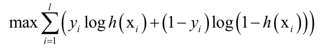
This is a convex optimization problem. You can use either the gradient descent method or the Newton method to solve it.
Logistic regression is a discriminative model. It should be noted that it is a linear model for binary classification problems.
Random forest

Core: Use samples with replacement sampling to train multiple decision trees. Each node of the training decision tree uses only part of the features of sampling without replacement. The prediction results of these trees are used for voting during prediction.

Random forest is an ensemble learning algorithm, which consists of multiple decision trees. These decision trees are trained by randomly sampling the training sample set to construct a sample set. Random forest not only samples the training samples, but also randomly samples the components of the feature vector. When training the decision tree, only a part of the sampled feature components are used as candidate features for splitting each time.
For classification problems, a test sample will be sent to each decision tree for prediction, and then voted. The class with the most votes is the final classification result. For regression problems, the predictive output of a random forest is the mean of the outputs of all decision trees.
Suppose there are n training samples. When training each tree, n samples are drawn from the sample set that have been replaced. Each sample may be selected multiple times, or it may not be drawn at once. Use this sampled sample set to train a decision tree. During training, each time the optimal split is searched, the components of the feature vector are also sampled, that is, only part of the feature components is considered.
Random forest is a discriminative model that supports classification problems, regression problems, and multiple classification problems. This is a non-linear model.
AdaBoost algorithm

Core: Use the linear combination of multiple classifiers to predict, focus on the samples that are misclassified during training, and the weak classifiers with high accuracy have more weight

The full name of the AdaBoost algorithm is Adaptive Boosting (Adaptive Boosting), which is an algorithm for binary classification problems. It uses a linear combination of weak classifiers to construct a strong classifier. The performance of weak classifiers is not too good, only stronger than random guessing, relying on them to construct a very accurate strong classifier. The calculation formula of the strong classifier is:
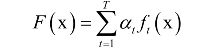
Where x is the input vector, F(x) is the strong classifier, ft(x) is the weak classifier, at is the weight of the weak classifier, T is the number of weak classifiers, and the output value of the weak classifier is +1 or -1, corresponding to positive samples and negative samples respectively. The judging rules for classification are:
sgn(F(x))
The output value of the strong classifier is also +1 or -1, which also corresponds to positive samples and negative samples.
When training, train each if classifier in turn, and get their weight value. Here, the training sample has a weight value. Initially, the weight of all samples is equal. During the training process, the sample that is misclassified by the previous weak classifier will increase the weight, otherwise it will decrease the weight, so that the next weak classification The processor will pay more attention to these difficult samples. The weight value of the weak classifier is constructed according to its accuracy. The higher the accuracy, the greater the weight of the weak classifier.
The AdaBoost algorithm is derived from the generalized additive model, and the minimum value of the exponential loss function is solved during training:
L(y, F(x)) = exp(-yF(x))
In the solution, a staged optimization is used to obtain the weak classifier first, and then determine the weight value of the weak classifier.
The standard AdaBoost algorithm is a discriminative model that can only support two classification problems. Its improved version can handle multiple classification problems.
Convolutional Neural Network

Core: a multi-layer composite function with shared weights

Convolutional neural network is also a multi-layer composite function in essence, but it is different from ordinary neural networks in that some of its weight parameters are shared, and another feature is that it uses a pooling layer. The back-propagation algorithm is still used during training, and the problem to be solved is not a convex optimization problem.
Like the fully connected neural network, the convolutional neural network is a discriminative model. It can be used for classification problems or regression problems, and supports multi-classification problems.
Recurrent neural network

Core: A function that combines compound functions and recursive sequences

The biggest difference from the ordinary neural network is that the cyclic neural network is a recursive sequence of numbers, so it has a memory function. Recall the arithmetic sequence we learned in high school:
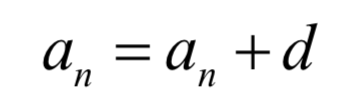
Once the first term a0 and tolerance d of the sequence have been determined, the following terms are also determined, so that the latter terms have no chance to change their own destiny at all. The cyclic neural network is also such a recursive sequence. The latter item is determined by the value of the previous item, but in addition, it also accepts a second input value, so that the output value this time is related to the previous sequence value. The input value at the current moment is related, and there is a chance to change your own destiny through the current input value:
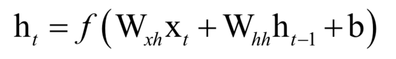
Like other types of neural networks, the cyclic neural network is a discriminative model, which supports not only classification problems, but also regression problems, and supports multi-classification problems.
K-means algorithm

Core: Assign the sample to the class to which the nearest class center belongs, and the class center is determined by all samples belonging to this class

The k-means algorithm is an unsupervised clustering algorithm. The algorithm assigns each sample to the class represented by the nearest class center, and the determination of the class center depends on the sample allocation plan. This is a question of whether the chicken comes first or the egg comes first.
In the implementation, first randomly initialize the class center of each class, then calculate the distance between the sample and the center of each class, assign it to the nearest class, and then recalculate the center of each class according to this allocation scheme. This is also a phased optimization strategy.
The problem to be solved by the k-means algorithm is an NPC problem, which can only be solved approximately, and there is a risk of falling into a local minimum.
Outdoor Rental LED Display is hot selling product in the led screen market. We usually use Nova MSD300 sending card and MRV328 receving card, other controll system also can be accepted, like Linsin,colorlight and so on.....About the led lamp, we use kinglight led lamp, IC is ICN2038S, refresh rate is 1920hz. We also provide other option if the client need higher quality, like Nationstar led lamp and refresh rate can make 3840hz. This 500x500mm LED display panel can also can make curved led display, ±15° flexible curved option.
Application:
* Business Organizations:
Supermarket, large-scale shopping malls, star-rated hotels, travel agencies
* Financial Organizations:
Banks, insurance companies, post offices, hospital, schools
* Public Places:
Subway, airports, stations, parks, exhibition halls, stadiums, museums, commercial buildings, meeting rooms
* Entertainments:
Movie theaters, clubs, stages.
Outdoor Rental LED Display,P3.91 Led Display,Led Advertising Display,Led Display Panel
Guangzhou Chengwen Photoelectric Technology co.,ltd , https://www.cwstagelight.com