
1. Establish a neural network add layer
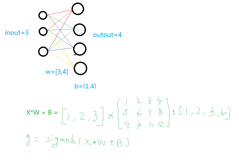
Input value, input size, output size, and excitation function
People who have studied neural networks can understand the following picture. If you don't understand, check out my other blog (http://).
Def add_layer(inputs , in_size , out_size , activate = None):
Weights = tf.Variable(tf.random_normal([in_size,out_size]))# random initialization
Baises = tf.Variable(tf.zeros([1,out_size])+0.1)# can be random but not initialized to 0, both are fixed values ​​better than random
y = tf.matmul(inputs, Weights) + baises #matmul: matrix multiplication, multipy: generally multiplication of quantities
If activate:
y = activate(y)
Return y
2. Train a quadratic function
Import tensorflow as tf
Import numpy as np
Def add_layer(inputs , in_size , out_size , activate = None):
Weights = tf.Variable(tf.random_normal([in_size,out_size]))# random initialization
Baises = tf.Variable(tf.zeros([1,out_size])+0.1)# can be random but not initialized to 0, both are fixed values ​​better than random
y = tf.matmul(inputs, Weights) + baises #matmul: matrix multiplication, multipy: generally multiplication of quantities
If activate:
y = activate(y)
Return y
If __name__ == '__main__':
X_data = np.linspace(-1,1,300,dtype=np.float32)[:,np.newaxis]#Creates a number of -1,1, 300, which is a one-dimensional matrix, which is later converted to a two-dimensional matrix == =[1,2,3]-->>[[1,2,3]]
Noise = np.random.normal(0,0.05,x_data.shape).astype(np.float32)#Noise is (1,300) format, 0-0.05 size
Y_data = np.square(x_data) - 0.5 + noise #Parabolic with noise
Xs = tf.placeholder(tf.float32,[None,1]) #外输入数æ®
Ys = tf.placeholder(tf.float32,[None,1])
L1 = add_layer(xs,1,10,activate=tf.nn.relu)
Prediction = add_layer(l1,10,1,activate=None)
Loss = tf.reduce_mean(tf.reduce_sum(tf.square(ys - prediction), reduction_indices=[1]))# error
Train_step = tf.train.GradientDescentOptimizer(0.1).minimize(loss)# Gradient optimization of the error with a step of 0.1
Sess = tf.Session()
Sess.run( tf.global_variables_initializer())
For i in range(1000):
Sess.run(train_step, feed_dict={xs: x_data, ys: y_data})# training
If i%50 == 0:
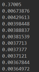
Print(sess.run(loss, feed_dict={xs: x_data, ys: y_data}))#View the error
3. Dynamic display of the training process
Some of the steps in the program are explained. For other instructions, please see other blogs (http://).
Import tensorflow as tf
Import numpy as np
Import matplotlib.pyplot as plt
Def add_layer(inputs , in_size , out_size , activate = None):
Weights = tf.Variable(tf.random_normal([in_size,out_size]))# random initialization
Baises = tf.Variable(tf.zeros([1,out_size])+0.1)# can be random but not initialized to 0, both are fixed values ​​better than random
y = tf.matmul(inputs, Weights) + baises #matmul: matrix multiplication, multipy: generally multiplication of quantities
If activate:
y = activate(y)
Return y
If __name__ == '__main__':
X_data = np.linspace(-1,1,300,dtype=np.float32)[:,np.newaxis]#Creates a number of -1,1, 300, which is a one-dimensional matrix, which is later converted to a two-dimensional matrix == =[1,2,3]-->>[[1,2,3]]
Noise = np.random.normal(0,0.05,x_data.shape).astype(np.float32)#Noise is (1,300) format, 0-0.05 size
Y_data = np.square(x_data) - 0.5 + noise #Parabolic with noise
Fig = plt.figure('show_data')# figure("data") specifies the chart name
Ax = fig.add_subplot(111)
Ax.scatter(x_data,y_data)
Plt.ion()
Plt.show()
Xs = tf.placeholder(tf.float32,[None,1]) #外输入数æ®
Ys = tf.placeholder(tf.float32,[None,1])
L1 = add_layer(xs,1,10,activate=tf.nn.relu)
Prediction = add_layer(l1,10,1,activate=None)
Loss = tf.reduce_mean(tf.reduce_sum(tf.square(ys - prediction), reduction_indices=[1]))# error
Train_step = tf.train.GradientDescentOptimizer(0.1).minimize(loss)# Gradient optimization of the error with a step of 0.1
Sess = tf.Session()
Sess.run( tf.global_variables_initializer())
For i in range(1000):
Sess.run(train_step, feed_dict={xs: x_data, ys: y_data})# training
If i%50 == 0:
Try:
Ax.lines.remove(lines[0])
Except Exception:
Pass
Prediction_value = sess.run(prediction, feed_dict={xs: x_data})
Lines = ax.plot(x_data,prediction_value,"r",lw = 3)
Print(sess.run(loss, feed_dict={xs: x_data, ys: y_data}))#View the error
Plt.pause(2)
While True:
Plt.pause(0.01)

4.TensorBoard overall structured display
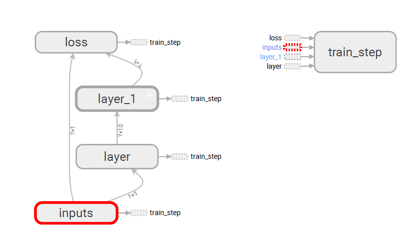
A. Create a large structure with with tf.name_scope("name") and create a small structure with the function name="name": tf.placeholder(tf.float32,[None,1],name="x_data")
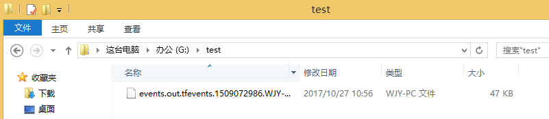
B. Create a graph file with writer = tf.summary.FileWriter("G:/test/",graph=sess.graph)
C. Use TessorBoard to execute this file
Here you have to pay attention --->>> first to the last directory where you store the file --->> and then run this file
Tensorboard --logdir=test
(Shielded GIF animation, specific installation operation welcome stamp "original link" Ha!)
5.TensorBoard local structured display
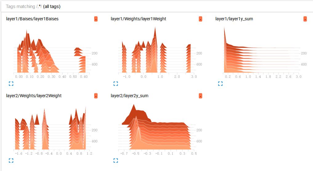
A. tf.summary.histogram(layer_name+"Weight", Weights): histogram display

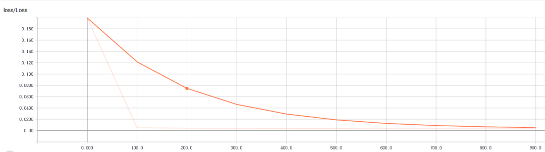
B. tf.summary.scalar("Loss",loss): The line chart shows that the direction of loss determines the quality of your network training, which is crucial.
C. Initialization and running settings chart
Merge = tf.summary.merge_all()#Merge chart 2 writer = tf.summary.FileWriter("G:/test/",graph=sess.graph)#Write to file 3 result = sess.run(merge,feed_dict= {xs:x_data,ys:y_data})#Run the packaged chart merge4 writer.add_summary(result,i)#Write the file, and the single step length is 50
Complete code and display effect:
Import tensorflow as tf
Import numpy as np
Import matplotlib.pyplot as plt
Def add_layer(inputs , in_size , out_size , n_layer = 1 , activate = None):
Layer_name = "layer" + str(n_layer)
With tf.name_scope(layer_name):
With tf.name_scope("Weights"):
Weights = tf.Variable(tf.random_normal([in_size,out_size]),name="W")#random initialization
Tf.summary.histogram(layer_name+"Weight",Weights)
With tf.name_scope("Baises"):
Baises = tf.Variable(tf.zeros([1,out_size])+0.1,name="B")# can be random but not initialized to 0, both are fixed values ​​better than random
Tf.summary.histogram(layer_name+"Baises",baises)
y = tf.matmul(inputs, Weights) + baises #matmul: matrix multiplication, multipy: generally multiplication of quantities
If activate:
y = activate(y)
Tf.summary.histogram(layer_name+"y_sum",y)
Return y
If __name__ == '__main__':
X_data = np.linspace(-1,1,300,dtype=np.float32)[:,np.newaxis]#Creates a number of -1,1, 300, which is a one-dimensional matrix, which is later converted to a two-dimensional matrix == =[1,2,3]-->>[[1,2,3]]
Noise = np.random.normal(0,0.05,x_data.shape).astype(np.float32)#Noise is (1,300) format, 0-0.05 size
Y_data = np.square(x_data) - 0.5 + noise #Parabolic with noise
Fig = plt.figure('show_data')# figure("data") specifies the chart name
Ax = fig.add_subplot(111)
Ax.scatter(x_data,y_data)
Plt.ion()
Plt.show()
With tf.name_scope("inputs"):
Xs = tf.placeholder(tf.float32,[None,1],name="x_data") #外输入数æ®
Ys = tf.placeholder(tf.float32,[None,1],name="y_data")
L1 = add_layer(xs,1,10,n_layer=1,activate=tf.nn.relu)
Prediction = add_layer(l1,10,1,n_layer=2,activate=None)
With tf.name_scope("loss"):
Loss = tf.reduce_mean(tf.reduce_sum(tf.square(ys - prediction), reduction_indices=[1]))# error
Tf.summary.scalar("Loss",loss)
With tf.name_scope("train_step"):
Train_step = tf.train.GradientDescentOptimizer(0.1).minimize(loss)# Gradient optimization of the error with a step of 0.1
Sess = tf.Session()
Merge = tf.summary.merge_all()# merge
Writer = tf.summary.FileWriter("G:/test/",graph=sess.graph)
Sess.run( tf.global_variables_initializer())
For i in range(1000):
Sess.run(train_step, feed_dict={xs: x_data, ys: y_data})# training
If i%100 == 0:
Result = sess.run(merge,feed_dict={xs:x_data,ys:y_data})#Run the packaged chart merge
Writer.add_summary(result,i)#write file, and single step 50
Guangzhou Chengwen Photoelectric Technology co.,ltd , https://www.cwledpanel.com